Example: Line Plot Example

\documentclass{minimal}
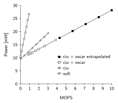
% Line plot example using external data fiels.
%
% Author: Claudio Favi
\usepackage{tikz}
\usetikzlibrary{plotmarks}
% The data files, written on the first run.
\begin{filecontents}{div_soft.data}
#MOPS 	Power [mW]
1.33E-02	10.403432
1.33E-01	12.53108
2.66E-01	14.90265
3.99E-01	17.22483
5.31E-01	19.58292
6.64E-01	21.89876
7.97E-01	24.44624
9.30E-01	26.6708
\end{filecontents}

\begin{filecontents}{div_ciu.data}
# MOPS 	Power [mW]
4.35E-02	9.562436
4.35E-01	10.845494
8.69E-01	12.24356
1.30E+00	13.66974
1.74E+00	15.13008
2.17E+00	16.57845
2.61E+00	17.97894
3.04E+00	19.41534
\end{filecontents}

\begin{filecontents}{div_ciu_oscar.data}
#MOPS 	Power [mW]
8.57E-01	11.255013
9.99E-01	11.4804
1.14E+00	11.718
1.29E+00	11.9916
1.64E+00	12.65854
2.00E+00	13.308
2.64E+00	14.484
3.85E+00	16.8
\end{filecontents}

\begin{filecontents}{div_ciu_oscar_extrapolated.data}
# MOPS 	Power [mW]
4.28E+00	17.56312023
5.71E+00	20.21127914
7.14E+00	22.85943805
8.57E+00	25.50759696
9.99E+00	28.15575587
\end{filecontents}

\begin{document}
\begin{tikzpicture}[y=.2cm, x=.7cm,font=\sffamily]
 	%axis
	\draw (0,0) -- coordinate (x axis mid) (10,0);
    	\draw (0,0) -- coordinate (y axis mid) (0,30);
    	%ticks
    	\foreach \x in {0,...,10}
     		\draw (\x,1pt) -- (\x,-3pt)
			node[anchor=north] {\x};
    	\foreach \y in {0,5,...,30}
     		\draw (1pt,\y) -- (-3pt,\y) 
     			node[anchor=east] {\y}; 
	%labels      
	\node[below=0.8cm] at (x axis mid) {MOPS};
	\node[rotate=90, above=0.8cm] at (y axis mid) {Power [mW]};

	%plots
	\draw plot[mark=*, mark options={fill=white}] 
		file {div_soft.data};
	\draw plot[mark=triangle*, mark options={fill=white} ] 
		file {div_ciu.data};
	\draw plot[mark=square*, mark options={fill=white}]
		file {div_ciu_oscar.data};
	\draw plot[mark=square*]
		file {div_ciu_oscar_extrapolated.data};  
    
	%legend
	\begin{scope}[shift={(4,4)}] 
	\draw (0,0) -- 
		plot[mark=*, mark options={fill=white}] (0.25,0) -- (0.5,0) 
		node[right]{soft};
	\draw[yshift=\baselineskip] (0,0) -- 
		plot[mark=triangle*, mark options={fill=white}] (0.25,0) -- (0.5,0)
		node[right]{ciu};
	\draw[yshift=2\baselineskip] (0,0) -- 
		plot[mark=square*, mark options={fill=white}] (0.25,0) -- (0.5,0)
		node[right]{ciu + oscar};
	\draw[yshift=3\baselineskip] (0,0) -- 
		plot[mark=square*, mark options={fill=black}] (0.25,0) -- (0.5,0)
		node[right]{ciu + oscar extrapolated};
	\end{scope}
\end{tikzpicture}
\end{document}